EET Algorithm using C++
For the purpose of my summer time project I was trying to write EET algorithm, for the task of planning the robot trajectory, from the scratch. According to my task requirements, I needed to write with the OMPL [4] interface so it could be easily implemented and tested alongside the existing algorithms in the OMPL library. All relevant information and all about the advantages of this algorithm read [1]. In the process I also attached and used some other libraries in my project, among them: Flexible collision library 0.5 [6] OpenMesh [5] In the very beginning, for understanding the Algorithm I used the publication [1]. As for some who wasn’t familiar with this publication, I would try to explain it here in order for you to better understand my work.
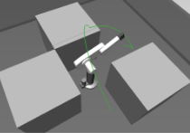
EET algorithm, at first, tries to determine the part of the space which should more likely have a path included from the start to the goal configuration. So in order to shrink the exploration space, it builds a sphere space configuration tree, which should in best way represent the parameters of the surrounding area shrank to the part of sphere tree in which robot is trying to find the path to the goal.
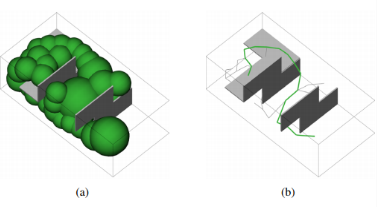
Figure 1. [1] On picture (a) you can see a sphere tree, and on the picture (b) a path found based on the configuration sphere tree
As input, algorithm has start and goal joint configurations.
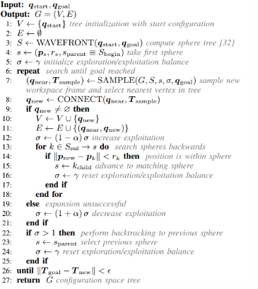
Figure 2. [1] EET algorithm, main part.
Output of the algorithm is the configuration space tree.
On the third line of the algorithm we are calling the function Wavefront in order to build a workspace sphere tree.
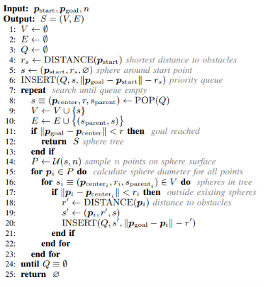
Figure 3. [1] WAVEFRONT function.
For input, function has workspace position of frame T, which determines the position of EOF joint configuration and also function is getting parameter n, which determines number of sampled points on the sphere surface.
So how does Wavefront work? Position of EOF is represented as a point, by the function DISTANCE (Figure 3) we get the distance to the closest point of the workspace. Then at the line 5 we are determining the sphere by its centre as a first argument, then radius as a previously calculated distance and by the parent sphere, which in this case is a zero sphere because our sphere is built around starting point. Then on line 6, we are inserting our sphere in the priority queue Q. Priority queue has spheres sorted by the parameter of absolute difference between start and goal point reduced by the sphere radius. The sphere in the first position will have the lowest value of that sorting parameter. Afterwards we are getting into the loop. At line 8 we are taking the first sphere from Q and simultaneously deleting it from the queue, all together with function POP. In lines 9 and 10 we are building the sphere tree, adding taken sphere to our vertices and adding edge between the parent and the current sphere. If the condition on the line 11 is satisfied it means that our end point is contained inside the sphere we just added to the sphere tree, so we can exit our loop. Otherwise, we are sampling n points on our last, added to sphere tree, sphere and for every point and for every contained sphere in the sphere tree, if our sampled point is out of some of the previous spheres in tree (in order for our tree to continuously expand forward), we calculate the distance from that point to the closest object in workspace and add this sphere to the priority queue in line 20 alongside the sorting parameter. And then if the ending condition is not satisfied (the priority queue became empty, if so, it means that our algorithm can’t find solution, and it returns empty tree) we are getting back to line 8 and doing it again all the way until we find solution or until we have no sphere in the priority queue, in which case it returns empty sphere tree.
Continuing further the algorithm, in the main part line 5, we are initializing the parameter for exploration/exploitation balance. Basically this parameter is responsible for the probability of sampling the point in some area around the sphere centre Figure 4.

Figure 4. [1] If the parameter is equal to 0, it means that it will always take the centre point, otherwise if it’s more than 0 but less than 1 it will proportionally to the sphere radius with bigger probability take some point at some distance from the centre according to the value of this parameter. And if it becomes more then 1 it means that it cannot find the solution of this kind within this sphere and the algorithm will go back to previous sphere trying to find different solution.
In line 6 in main we are getting into the loop. Starting the loop with the sampling of position and orientation and determining closest joint configuration on line 7 in main part, by calling the function Sample.
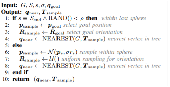
Figure 5. [1] Function SAMPLE. In line 1, if probability of sampling the goal state is satisfied then as a position and orientation we are taking the position and orientation of the given goal. Else, we are sampling position within sphere (using exploration/exploitation parameter) and doing uniform sampling for orientation. Based on that by function NEAREST we are determining the nearest vertex in tree (most convenient for already determined joint orientation) to be continued to the sampled position and orientation.
Then in the main part in line 8 we are determining new joint configuration by the function CONNECT.
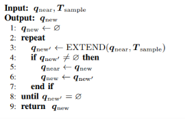
Figure 6. [1] Function CONNECT. Initializing new joint configuration as the new element, line 1. Getting into the loop in line 2, which we will exit only if new buffer joint configuration becomes equal to 0(it’s marked with the apostrophe). In line 3 we are getting the value of buffer joint configuration with function Extend. Checking whether the element is empty or we have solution, if we have solution, we are replacing the nearest joint configuration with a previous value of new joint configuration, then new joint configuration is getting value of buffer joint configuration (which we got in the function EXTEND) then we will do this all again, this way we will be able to find the most effortless solution for the robot to come from the start to its goal position.
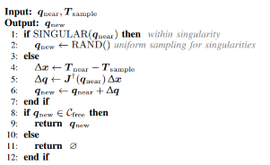
Figure 7. [1] Function EXTEND. Giving the nearest joint configuration and sample position and orientation in the first line we are checking whether it is within singularity, if so we are taking random joint orientation for new joint configuration. Otherwise we are determining the difference between orientation and position of EOF of nearest joint configuration and sampled one. Based on that we are solving inverse kinematic problem and determining new joint configuration. Further on, on line 8 we are checking whether there are any collisions and returning new configuration, otherwise returning empty element.
Returning back to the main algorithm. On line 9, if we got new joint configuration, we are adding it to our tree. Then on line 12 we will increase exploitation (it means that we will sample points closer to the sphere centre). On line 13 for spheres in sphere tree, starting backwards, checking whether new position is within some other than the last sphere, if it is, we will advance to that sphere and we will continue from there (it’s done for the path optimisation). If we didn’t get new joint configuration in line 8, we will advance to line 20, decrease exploitation, check whether is bigger than 1 (if it is, we will reset it to default value and we will go back to the previous sphere, and try to find another solution), then we will go through the loop again until difference between our new and goal position and orientation is less than given threshold value for goal state comparison.
Review of the work done. For my summer project, I was able to do the part of the algorithm and check how it works. I was able to visualize the results and I will explain everything and show the results. My project was done at CLION at version for the students; there was no intention to use this for any other then education purposes.
As I mentioned previously in order to have OMPL interface for my algorithm, I called my base part as Base_OMPL, where my main.cpp is contained. In main.cpp file I am defining everything I need for the space configuration, loading the model which is taken from OMPLapp BugTrap_planar_env.ply.
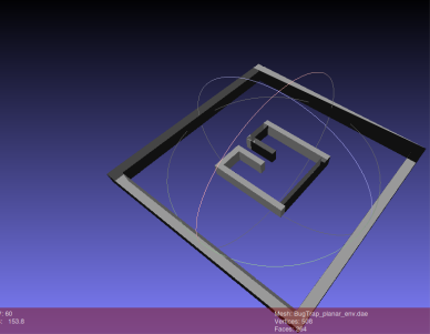
Picture 1. BugTrap_planar_env.ply
The bounds which I wrote in main.cpp I added knowing the environment I was loading from file. As the validity checker I set up the FCL library, so everything regarding the part for collision checking and calculating closest distance to collision I am doing using FCL library. I am making a sphereTree object, which as a result calculates the sphere tree. For representation of start and end points I am using Eigen library. Currently I am calculating for the predefined points. Then I am printing the result using OpenMesh library, as it was most convenient library to work with the workspace and also with the result representation.
Part which I compiled as a library, added to my base part, responsible for building Sphere Tree is contained in folder Sphere-handle in my project. Sphere approximation is written based on explanation given on the website [2], where the code was written using python. This part is done for the ability to visualize the result of my program, so every sphere calculated is then added to my OpenMesh file, calculation of the base sphere with radius 1 and centre in the 0 is done only once, for all other spheres to be calculated just multiplication and translation is done. WorkspaceSphere files are taken from [3]; they have been modified and adjusted to my program. Here alongside the criteria presented in [1] there are two more. All they are called: GREEDY_DISTANCE, GREEDY_SOURCE_DISTANCE, and GREEDY_SPACE. The tree is represented using BOOST library.
So to be able to manipulate with workspace, as I wrote, I am using OpenMesh. But in order to work with a workspace I am using FCL. So part responsible for converting, which is also added to the base part as a library is written in folder Parse_OpenMesh>FCL. In function model I am doing the iteration through every face and every vertex and then make FCL model.
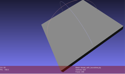
Picture 2. BugTrap_planar_env.ply with boundaries.
There with the function add_boundaries_for_bagtrap I am adding 4 additional triangles which are determined specificly for this model in order for my planner not to exceed the workspace parameters. In simple words I am putting my workspace in a box and then giving it to the FCL.
Part with FCL is contained in FCL_STATE_CHECK; it’s also added as a library to the other parts. At first I was trying to initialize dummy collision object(The dot, as a simplest object possible) but then it was clear that my current version of currently installed library doesn’t support this kind of object, and I decided to represent dot as a sphere object with really small radius(of course compared to my workspace) according to my needs. Here I am determining two functions one is validity state checker and another is distance to collision.
As for the end, in summary, setting up everything with OMPL, taking and manipulating data with OpenMesh, working with data using FCL I am getting the sphereTree build. For visualisation I am opening the written files using MeshLab.
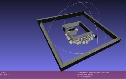
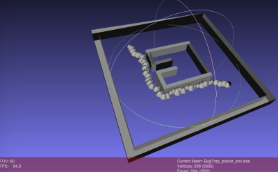
Picture 3 and 4. Solutions with different start (black sphere) and end points
[1]Balancing Exploration and Exploitation in Sampling-Based Motion Planning Markus Rickert, Arne Sieverling, and Oliver Brock http://www.robotics.tu-berlin.de/fileadmin/fg170/Publikationen_pdf/Rickert-14-TRO.pdf
[2]Triangulating a Sphere Recursively https://sites.google.com/site/dlampetest/python/triangulating-a-sphere-recursively
[3]Copyright (c) 2009, Markus Rickert https://github.com/roboticslibrary/rl/blob/a3f035ccb571e97dcac7257b5e5dd9f6a0d860f6/src/rl/plan/Eet.cpp
[4]OMPL http://ompl.kavrakilab.org/
[5]OpenMesh https://www.openmesh.org/
[6] Flexible Collision library https://github.com/flexible-collision-library